This is work in progress. It is liable to change from day to day.
A benefit of sexual reproduction
This document aims to answer the question "What is the advantage of sexual reproduction, that compensates for the twofold disadvantage?
Contents
History of the problem
Consider a female who will give birth to n progeny. If she can choose between producing n progeny identical to herself and n each carrying half her genes and half the genes provided by a male, the former seems clearly more in her genetic interests. Yet most higher animals and plants, including almost all mammals, use sexual reproduction every generation. This needs explaining.
Many explanations have been offered, particularly in the 1970s. These included the "aphid rotifer", "strawberry-coral", and "elm-oyster" models[A], the "tangled bank" idea[B], the "libertine bubble" idea[C], and the "Red Queen hypothesis"[D]. More recent ideas have been the counteracting of Muller's ratchet[E], the "removal of minor faults"[F], the possibility of providing an unbounded rate of information gain[G], and its rôle in the host-parasite arms race[H].
Most studies, both experimental and theoretical, have concentrated on relatively high selective pressures. For experiments, this is clearly necessary. We concentrate on low selective pressures, at many loci, using a computer model described below. We believe this clarifies a major benefit of sexual reproduction, in a way which is compatible with many of the hypotheses listed above.
Description of the model
show
A population is modelled as a 2-dimensional array, one dimension representing the members of the population and the other the loci currently with two alleles present in the population. Each member of the array is the number of copies of the "new" allele for that locus present in that individual: 0 or 1 for haploid populations, 0, 1 or 2 for diploid populations.
Each generation, a user-specified mutation rate is applied. There are two options for how this is done:
-
Fixed number of loci.
The number of loci is user-specified. We assume that all mutant alleles at any one locus have the same fitness, and that there are no reverse mutations. The fitness of a new allele is drawn from a user-specified p.d.f.
-
Infinite number of loci.
Every mutation is at a different locus, with a fitness drawn from a user-specified p.d.f. (This uses less computer memory than a model with a large fixed number of loci.)
In a diploid or "sexual haploid" population, the individuals "breed" every generation; or only every m generations if this is specified by the user. This is represented by every individual producing a number of gametes, with a Poisson distribution whose mean is proportional to its total fitness (the product of the fitnesses of all it alleles).
The gametes are stored in an array, in their order of creation. If the population is specified as panmictic, it is then shuffled. Then the gametes are paired up using a "cut-and-slide" algorithm, to produce new individuals, which are stored in the main array, again in the order of their creation. In a diploid population, each new individual has two complete gametes, in a "sexual haploid" population each new individual is assigned an allele at each locus randomly and independently from each of its two parent gametes (there is no linkage). The use of independent Poisson distributions results in a population of a size varying slightly from what was specified; this is counteracted by choosing an adjusted target size for the following generation.
Explanation of the graphs
show
Each of the graphs presented in the these pages shows the effect of computer-simulated selection on a population, by plotting the frequencies of new alleles. The selective force acting on the alleles in these simulations is very low, while the number of generations is high.
For each graph, the horizontal axis shows the number of generations since the start of the simulation. The graph is typically not plotted every generation; in the pages that follow it is plotted every 5, 10, or 25, generations.
The vertical axis shows the proportion of the new alleles in the population. If a new allele is favoured by selection, this is seen rising from 0 to 1 (fixation). If a new allele becomes extinct (because it is disadvantageous, or through drift), the graph rises and then falls back to 0 (extinction of the allele). To make the graphs clearer, alleles whose frequency never reach some cutoff frequency (0.005 in the following pages) are not plotted.
Each graph also includes
- a red line, showing the mean fitness of the population (on a log scale, as fitnesses are treated as multiplicative)
- a green line, showing the variance of the population, which can be regarded as a measure of the rate of selective deaths
- vertical green lines, indicating the interval within which statistics for the number of alleles fixed and for cumulative variance are collected
The values of various parameters that influence the selection are written on the graphs. In order from left to right along the top of the graphs, they are:
- The file name.
- (asexual) haploid, sexual haploid; diploid (not yet supported).
- "mixing": whether the breeding is panmictic (1), or with minimal movement (0). For haploid populations, this is omitted as irrelevant.
- "breed_at": the number of generations between sexual generations. "1" means every generation. For haploid populations, this may be omitted as irrelevant.
- "n": the population size.
- "a": a Perl function defining the distribution of the new alleles. For example, "a=1.01" means "all new alleles have fitness 1.01"; "a=rand(1.1)" means "fitnesses rectangular in the range 0—1.1"; and "a=1+rand(0.1)" means "fitnesses rectangular in the range 1—1.1".
- "μ": the mutation rate per individual per generation (if the number of loci is infinite); or per individual per generation per locus(if the number of loci is specified).
- "loci": the number of loci.
- "seed" is a seed for the simulations random number generator.
The number of new alleles fixed in the simulation is shown on the graph itself, at the top left corner. The count starts only after the simulation has run for some number of generations (typically 500), as indicated by a vertical green line on the graph.
Interpretation of the graphs
hide

Above is a sample graph, for a haploid population. The population size is 2000, the mutation rate is 0.001 per individual per generation, and the finesses of mutant alleles is rectangularly distributed between 0 and 1.1 (so most are disadvantageous).
The first four alleles to achieve a frequency of over 0.1 all rise smoothly to fixation, in sigmoid shapes. The first of these becomes fixed in about generation 250, to the left of the green line, so is not inluded in the total "Fixed 7".
The fifth allele to rise above 0.1 frequency peaks at about 0.14, and then rapidly falls back to 0 because it is competing with a new and fitter allele which appeared at another locus in generation 600. Then that new and fitter allele itself starts to fall back, because of competition from two more new alleles. But after falling to a frequency just below 0.6, it starts to rise again. This is because yet another fit new allele, arising in an individual which already had the "generation 600" allele, helps it to compete. (We can tell that it did so because the graphs for the two alleles eventually merge at generation 920: thereafter all the individuals that have the generation-600 allele also have its accomplice).
When looking at a graph for an asexual population, we often see two lines merge into a single line. This happens when the more recent and rarer of the two alleles has appeared in an individual already having the older allele. Also, with an asexual population, we often see two lines "mirror" each other: wherever one rises, the other falls by the same amount, as at generations 700 to 900 in the graph above. This happens when the entire population carries one or another of the alleles, but not both. The two lines continue to rise and fall, not only because of drift, but because of the appearance of other new alleles within one or the other of the two subpopulations.
The paragraph above is italicised because it is a key to understanding these graphs. The merging, and to some extent the mirroring, are also seen in graphs for sexual populations, but are less prevalent there.

Above is a graph with the same parameters as the previous one, except that it is for a sexual population. It shows similar sigmoid ascents, but with the difference that rather than "competing", two of the sigmoids can continue upwards together. We see a low-slope sigmoid, that achieves 0.5 frequency in generation 325, continue its slow upwards progress while being overtaken by other newer and fitter alleles. Unlike in the haploid case, the appearance of fitter alleles at other loci is not a setback for it, instead, individuals carrying both beneficial alleles are generated by sex.
Some results
1. Haploid compared with sexual haploid
Using pairs of graphs such as those shown in the previous section, but run for more
generations, we see that new alleles achieve fixation at a higher rate in a "sexual haploid" population than in a haploid population.
show graphs
2. Panmictic compared with unmixed
If we compare a panmictic sexual haploid population with a sexual haploid population without mixing (the individuals are treated as being in a line, each pairs with one of the adjacent individuals), we find that the former has new alleles achieving fixation at a higher rate. Both do better than a haploid population (for which mixing has no effect).
show graphs
3. With and without adverse mutations
We compare the effect of having adverse mutations (the fitness of a new allele is rectangular in the range 0 to 1.1) and having no adverse mutations (the fitness of a new allele is rectangular in the range 1 to 1.1, and the total mutation rate is 1/11 as much). We find that there is no significant difference in the rate of fixation of new alleles, in both sexual haploid and haploid simulated populations. However, the variance in the fitness of evolving populations is higher if there are adverse mutations.
show graphs
4. The effect of population size
In both haploid and sexual haploid populations, the rate of fixation of new alleles is higher in larger populations. This effect of population size is greater in sexual haploid than in haploid populations.
show graphs


 Rows: population size is 100, 200, 500, 1000, 1500, 2000, 3000, 4000, 5000.
Left column: sexual haploids.
Right column: haploids.

Population
size | Alleles fixed,
sexual haploids | Alleles fixed,
true haploids |
|---|
| 100 | 5 | 6 |
| 200 | 8 | 9 |
| 500 | 7 | 22 |
| 1000 | 23 | 39 |
| 1500 | 28 | 56 |
| 2000 | 35 | 71 |
| 3000 | 46 | 102 |
| 4000 | 49 | 111 |
| 5000 | 47 | 130 |
The graph to the right is of the log of the rate of fixation of new alleles against the log of the population size, for haploid "hap" and sexual haploid "sh" populations. Their slopes are about 0.55 and 0.8 respectively.
5. The effect of a finite number of loci
In both haploid and sexual haploid populations, the rate of fixation of new alleles is higher in larger populations. This effect of population size is greater in sexual haploid than in haploid populations.
show graphs
We see that effects described above with an infinite number of loci are still seen when the number is finite.
In the lower half of the graphs in this section, with the fitnesses of new alleles randomly chosen in the range 0 – 1.1, most of these alleles will be deleterious and very rarely achieve fixation. So the number that are ever likely to be fixed is limited to approximately 1/11 of the number of loci.
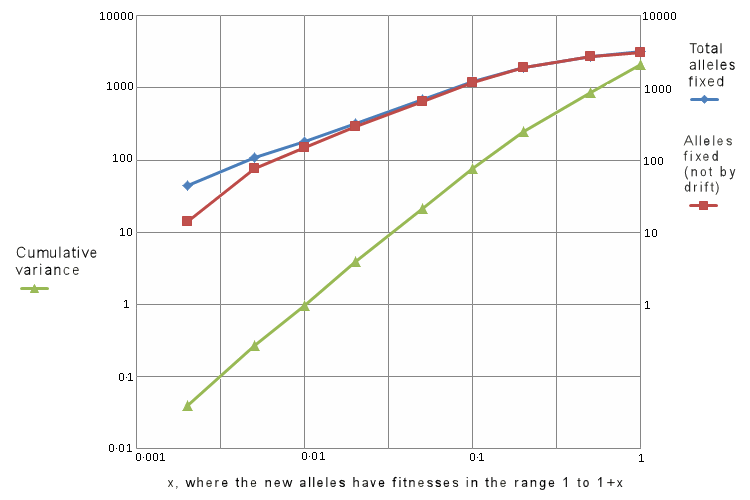
6. The efficiency of low selection rates
We compare the effect of fitnesses of new alleles in the range 1 – x, with x varying from 0.1 to 0.00001. For each value, over sexual haploid populations of size 1000 with infinite loci, we examine the number of new alleles fixed and the cumulative log variance of the fitness. The latter is a measure of the cumulated rate of selective deaths in the evolving population.
show graphs
Only six of sixteen graphs are shown below, because they are they are large files, typically about 4MB each, and display all sixteen at once would impose a heavy load on a browser. Links are provided for the other ten.
a=1+rand(1), 3162 alleles fixed
a=1+rand(0.5), 2752 alleles fixed
a=1+rand(0.2), 1949 alleles fixed
a=1+rand(0.1), 1217 alleles fixed
a=1+rand(0.05), 688 alleles fixed
a=1+rand(0.02), 326 alleles fixed
a=1+rand(0.01), 181 alleles fixed
a=1+rand(0.005), 107 alleles fixed
a=1+rand(0.002), 44 alleles fixed
a=1+rand(0.001), 24 alleles fixed
a=1+rand(0.0005), 29 alleles fixed
a=1+rand(0.0002), 30 alleles fixed
a=1+rand(0.0001), 38 alleles fixed
a=1+rand(0.00005), 31 alleles fixed
a=1+rand(0.00002), 31 alleles fixed
a=1+rand(0.00001), 22 alleles fixed


| x |
Number of new
alleles fixed |
Number of new
alleles fixed
not by drift |
Cumulative variance
of log of fitness |
|---|
| 1 | 3162 | 3132 | 2096 |
|---|
| 0.5 | 2752 | 2722 | 872 |
|---|
| 0.2 | 1949 | 1919 | 249 |
|---|
| 0.1 | 1217 | 1187 | 77.4 |
|---|
| 0.05 | 688 | 658 | 21.65 |
|---|
| 0.02 | 325 | 295 | 3.94 |
|---|
| 0.01 | 181 | 151 | 0.98 |
|---|
| 0.005 | 107 | 77 | 0.27 |
|---|
| 0.002 | 44 | 14 | 0.040 |
|---|
| 0.001 | 24 | – | 0.010 |
|---|
| 0.0005 | 29 | – | 0.0024 |
|---|
| 0.0002 | 30 | – | 0.00047 |
|---|
| 0.0001 | 38 | – | 0.000092 |
|---|
| 0.00005 | 31 | – | 0.000044 |
|---|
| 0.00002 | 31 | – | 0.000004 |
|---|
| 0.00001 | 22 | – | 0.000001 |
|---|
We see that for low selection rates, the number of new alleles fixed does not depend on the selection rate, but is constant at about 30. These alleles are being fixed by drift rather than by selection. Therefore we have created a column in the table above for new alleles fixed other than by drift, being 30 less than the number fixed.
The coloured graph to the right shows the number of alleles fixed (both in total, and not by drift) and the total variance of the fitnesses, against the selective force x, all on log scales. The total variance is a measure of the selective death rate, being proportional to its square.
We see that within the range 0.05 < x < 0.1, the graphs are straight lines, with slopes of about 0.9 for the alleles fixed, and 1.9 for the total variance.
Thus we have, for the conditions of these simulations:
No. of alleles fixed is proportional to x0.9
Total variance in fitness is proportional to x1.9
7. Finite and infinite loci
Do these simulation for an infinite number of loci give the same results as for a number large enough not to "run out" in the course of the simulation?
show graphs
We see that the simulations with infinite loci have very similar results to those with infinite loci. So our code treats "an infinite number of loci" in the same way as "a very large number of loci".
We also see that for the lowest mutation rate, 0.05 mutations per individual per generation, the fixation rate is higher for haploids than for sexual haploids. This may be because with sexual haploids, each new allele spreads very slowly, not much faster than it would by drift, and very few are fixed in the course of this simulation; whereas in a haploid population, several beneficial mutations that happen to occur in the same bloodline can rise together at a significantly faster rate than drift, without being separated by sexual reproduction.
Conclusions
From the comparisons above, specifically Haploid compared with sexual haploid and The effect of population size, we conclude that
Acquiring a new allele very slowly is very efficient in selective deaths.
Acquiring mutliple new alleles at once, all very slowly, is very efficient only if the acquisitions do not interact negatively with each other, as they do in asexual populations. Sexual reproduction reduces negative interactions. Frequent sexual reproduction combined with panmixis prevents negative interactions.
Further questions to consider
show
What is the "cost of evolution"?
If we define a measure of cost, such as selective death rate, how many genes per generation can be pushed through to fixation, as a function of the measure?
We suspect that, for large population size, it is unbounded.
Real evolution will always fall well short of the theoretical best attainable value. Potential opportunities for evolution will be wasted, e.g. in maintained balanced polymorphisms, and in cyclic evolution (such as one phenotype being favoured in the summer, another in the winter).
What proportion of generations "should" be sexual?
In a population with optional sexual reproduction, how can we estimate its optimal frequency? What proportion of generations should be sexual? Is there a trade-off, with infrequent sex favoured in the short term and frequent sex in the long term?
Reticulated population structure
Is a "reticulated" population structure more favourable to evolution than a panmictic structure? (i.e., instead of one large panmictic population, a set of smaller panmictic populations, with occasional exchanges of individuals among them?
References
[A]
George C. Williams. 1975. Sex and Evolution, Princeton University Press
[B]
Graham Bell. 1982. The Evolution and Genetics of Sexuality. University of
California Press, Berkeley.
[C]
Thierry Lodé. 2011. Sex is not a good solution for reproduction: the libertine bubble theory. Bioessay 33: 419–432
[D]
Leigh Van Valen. 1973. "A new evolutionary law". Evolutionary Theory. 1: 1–30.
[E]
Hermann Joseph Muller. 1932. "Some genetic aspects of sex". American Naturalist. 66 (703): 118–138
[F]
Alexey Kondrashov. 1988. "Deleterious mutations and the evolution of sexual reproduction". Nature 336: 435-440
[G]
David J.C. MacKay. 2003. Information Theory, Inference, and Learning Algorithms, C.U.P. 2003: chapter 19.
http://www.inference.org.uk/itprnn/book.pdf
"An information theoretic analysis using a simplified but useful model shows that in asexual reproduction, the information gain per generation of a species is limited to 1 bit per generation, while in sexual reproduction, the information gain is bounded by sqrt(G}, where G is the size of the genome in bits."
[H]
Lively & Morran. 2014. The Ecology of Sexual Reproduction. Journal of Evolutionary Biology, 1292-1303
doi: 10.1111/jeb.12354
Copyright N.S.Wedd 2018.


